Concavity Explorer

Understanding the Shape of Functions

∪

Concave Up

Watch a sphere settle into a concave bowl, just like a parabola curving upward

∩

Concave down (convex)

See a sphere roll off a convex surface, mirroring a downward-curving function

y = 1+x²

Tangents to Concave Up

Visualize tangent lines sweeping across a concave upward curve

y = 1-x²

Tangents to Convex

See tangent lines moving across a concave down (convex) curve

f''(x) > 0

Concave Mathematics

Explore the mathematical theory behind concave upward functions

f''(x) < 0

Convex Mathematics

Understand the mathematics of concave down (convex) surfaces

📊

Summary of f''(x) and curvature

A comprehensive overview of second derivatives, concavity, and inflection points

Concave Up Animation

A sphere rolling in a concave bowl settles at the minimum point

Concave down (convex) Animation

A sphere rolling off a convex surface demonstrates instability at the maximum

Tangents to Concave Up Curve

The tangent always lies below the curve. The slope of the tangents increase from negative, through zero, to positive.

Tangents to Convex Curve

The tangent always lies above the curve. The slope of the tangents decrease from positive, through zero, to negative.

Mathematics of Concave Up Functions

When the graph curves upward like a smile

Definition

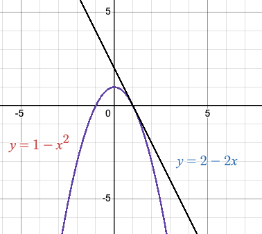
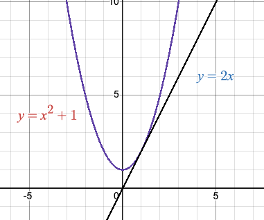
A function y = f(x) is concave up (or concave upward) on an interval if the graph of the function lies above all of its tangent lines on that interval. Visually, the graph curves upward, resembling the shape of a bowl or the letter "U".

Key Insight: For a concave up function, the rate of change is increasing. As you move from left to right, the slope of the tangent line becomes steeper (more positive or less negative).

Graph and second derivative

For a concave up region of a curve the gradient of the curve/tangent changes from negative to positive. For this region the graph of the gradient (derivative) is increasing (from negative to positive). Hence the gradient curve has itself a positive gradient, that is, the second derivative is positive.

Second Derivative Test

The primary mathematical test for concavity uses the second derivative:

If f''(x) > 0 for all x in an interval, then f is concave up on that interval

The second derivative f''(x) measures the rate of change of the first derivative f'(x). When f''(x) is positive, the slope is increasing, creating the upward curve.

EXAMPLE: f(x) = x²

First derivative: f'(x) = 2x

Second derivative: f''(x) = 2

Since f''(x) = 2 > 0 for all x, the parabola y = x² is concave up everywhere. The vertex at (0,0) represents a minimum point.

Physical Interpretation

Think of the concave up bowl in the animation. When the sphere is placed anywhere in the bowl, gravity pulls it toward the lowest point. This represents a stable equilibrium—any small displacement results in a force that returns the object to the minimum.

In calculus terms, at a critical point where f'(x) = 0, if f''(x) > 0, then that point is a local minimum. The concave up shape ensures that nearby points have higher function values.

Inflection Points

A function changes from concave up to concave down (convex) (or vice versa) at an inflection point. At these points:

f''(x) = 0 and f''(x) changes sign

EXAMPLE: f(x) = x³

First derivative: f'(x) = 3x²

Second derivative: f''(x) = 6x

• When x < 0: f''(x) < 0 (concave down (convex))

• When x > 0: f''(x) > 0 (concave up)

The point (0,0) is an inflection point where concavity changes.

Applications

Optimization: In economics, a concave up cost function indicates increasing marginal costs—each additional unit becomes more expensive to produce.

Motion: If position s(t) has s''(t) > 0, the object is speeding up in the positive direction (or slowing down less quickly in the negative direction).

Data Analysis: Concave up curves in data suggest accelerating growth, such as exponential population growth or compound interest effects.

Mathematics of Concave down (convex) Functions

When the graph curves downward like a frown

Definition

A function y = f(x) is concave down (convex) on an interval if the graph of the function lies below all of its tangent lines on that interval. Visually, the graph curves downward, resembling an upside-down bowl or the letter "∩".

Key Insight: For a concave down (convex) function, the rate of change is decreasing. As you move from left to right, the slope of the tangent line becomes less steep (less positive or more negative).

Note on terminology: In some contexts, especially in economics and optimization theory, "concave" without a modifier refers to what we call "concave down (convex)." A function that is concave down (convex) is also called "convex" in the sense of having a convex upper boundary. However, in calculus, we typically use "concave up" and "concave down (convex)" to avoid confusion.

Graph and second derivative

For a concave down (convex) region of a curve the gradient of the curve/tangent changes from positive to negative. For this region the graph of the gradient (derivative) is decreasing (from positive to negative). Hence the gradient curve has itself a negative gradient, that is, the second derivative is negative.

Second Derivative Test

The mathematical test for concave down (convex) behavior uses the second derivative:

If f''(x) < 0 for all x in an interval, then f is concave down (convex) on that interval

When f''(x) is negative, the first derivative f'(x) is decreasing. This means the slope of the function is getting smaller (less steep), creating the downward curve.

EXAMPLE: f(x) = -x²

First derivative: f'(x) = -2x

Second derivative: f''(x) = -2

Since f''(x) = -2 < 0 for all x, the inverted parabola y = -x² is concave down (convex) everywhere. The vertex at (0,0) represents a maximum point.

Physical Interpretation

Consider the convex bowl in the animation (opening downward). When the sphere is placed on top, any slight disturbance causes it to roll away. This represents an unstable equilibrium—the sphere cannot remain at the peak and will naturally move toward lower positions.

In calculus, at a critical point where f'(x) = 0, if f''(x) < 0, then that point is a local maximum. The concave down (convex) shape ensures that nearby points have lower function values, making the critical point a peak rather than a valley.

Comparison with Concave Up

The key differences between concave up and concave down (convex) functions:

CONCAVE UP (f''(x) > 0)

• Graph curves upward (∪ shape)

• Slope is increasing

• Critical points are local minima

• Stable equilibrium in physical systems

• Graph lies above tangent lines

CONCAVE DOWN (CONVEX) (f''(x) < 0)

• Graph curves downward (∩ shape)

• Slope is decreasing

• Critical points are local maxima

• Unstable equilibrium in physical systems

• Graph lies below tangent lines

Practical Examples

Projectile Motion: The height of a thrown ball follows a concave down (convex) parabola. After reaching maximum height, the ball descends. The concave down (convex) shape reflects constant downward acceleration due to gravity.

EXAMPLE: h(t) = -4.9t² + 20t + 2

This represents height (in meters) as a function of time (in seconds).

h'(t) = -9.8t + 20 (velocity)

h''(t) = -9.8 < 0 (acceleration due to gravity)

The negative second derivative confirms the concave down (convex) parabola, with maximum height occurring when h'(t) = 0.

Diminishing Returns: In economics, a concave down (convex) production function indicates diminishing marginal returns—each additional input produces less additional output than the previous input.

Learning Curves: Skill acquisition often follows a concave down (convex) curve initially—rapid improvement at first, then slower progress as one approaches mastery.

The Second Derivative Test for Extrema

Concavity is essential for classifying critical points:

Given a critical point c where f'(c) = 0:

If f''(c) > 0: concave up → local minimum at x = c
If f''(c) < 0: concave down (convex) → local maximum at x = c
If f''(c) = 0: test is inconclusive

This test provides a quick way to classify extrema without analyzing the first derivative on both sides of the critical point.

Summary of f''(x) and curvature

A comprehensive overview of second derivatives, concavity, and inflection points

The Big Picture

The second derivative f''(x) tells us about the curvature or concavity of a function. It measures how the rate of change (first derivative) is itself changing.

Core Concept: While f'(x) tells us if a function is increasing or decreasing, f''(x) tells us if that rate of increase/decrease is itself speeding up or slowing down.

Sign of f''(x) and Concavity

f''(x) > 0 → CONCAVE UP (∪ shape)
• The curve bends upward
• The slope f'(x) is increasing
• The graph lies above its tangent lines
• Examples: y = x², y = eˣ, y = x⁴

f''(x) < 0 → CONCAVE DOWN (∩ shape)
• The curve bends downward
• The slope f'(x) is decreasing
• The graph lies below its tangent lines
• Examples: y = -x², y = ln(x), y = -x⁴

f''(x) = 0 → POSSIBLE INFLECTION POINT
• Concavity may change at this point
• Must verify that f''(x) changes sign
• Could also be a "flat spot" in curvature without changing

Inflection Points: When Concavity Changes

An inflection point occurs where the curve changes from concave up to concave down (or vice versa).

Requirements for Inflection Point at x = a:

1. Function is continuous at x = a
2. f''(a) = 0 (or f'' is undefined)
3. f''(x) changes sign at x = a

Two Types:

• Horizontal inflection: f'(a) = 0 and f''(a) = 0
Example: f(x) = x³ at x = 0

• Non-horizontal inflection: f'(a) ≠ 0 and f''(a) = 0
Example: f(x) = x³ - 3x at x = 0

Quick Reference Table

Condition	f'(a)	f''(a)	Classification
Standard minimum	= 0	> 0	Local minimum
Standard maximum	= 0	< 0	Local maximum
Flat minimum (x⁴)	= 0	= 0	Local minimum (check f⁽⁴⁾ > 0)
Flat maximum (-x⁴)	= 0	= 0	Local maximum (check f⁽⁴⁾ < 0)
Horizontal inflection (x³)	= 0	= 0	Inflection point (f'' changes sign)
Sloped inflection	≠ 0	= 0	Inflection point (f'' changes sign)
Concave up region	any	> 0	Curve bends upward
Concave down region	any	< 0	Curve bends downward

Key Takeaways

Remember:
• f' tells you direction (increasing/decreasing)
• f'' tells you curvature (how direction is changing)
• f''(x) > 0 means curving up (∪), f''(x) < 0 means curving down (∩)
• f''(a) = 0 is a candidate for inflection, but must verify sign change
• Not all inflection points have horizontal tangents
• When second derivative test fails (f'' = 0), use alternatives